
Solving a problem is often easy. In schools, we learn various techniques that help us find solutions in different cases.
However, in day-to-day business, we realize that, unlike the way we learned, no one will hand you a pre-formulated problem. "Find the x" exists only in classrooms. What we find are data, signals, behaviors that need to be investigated for hypothesis generation and model adjustments.
Metrics / KPIs help us understand, for example, the operational deficiencies. Values are compared with values from other similar companies (benchmarks), but in many cases, if not all, the metrics will not indicate what the solution to the problem is.
If I could give one piece of advice to newcomers in the job market, I would recommend studying one of the most used statistical techniques in data analysis: linear regression.
In light of this, I decided, this month, to create this post aimed at explaining the fundamentals of the regression technique using the least squares method. I will also show how to manually calculate the adjusted equations in Excel.
I will not go into the significance analyses of models (F test of regression and t test of the parameters). This topic will be addressed in a future post. The idea is to show the concept and the understanding mathematical of this technique.
Just to exemplify, we will formulate some simple problems that are present in the day-to-day of companies.
Let's initially move to the conceptual part...
What is linear regression?
Linear Regression is a statistical technique
that fits a mathematical equation to the data to estimate the behavior of a
variable  based
on one or more variables
based
on one or more variables  .
.
The term 'linear' in regression refers to the way
coefficients enter the equation, and not to the geometric shape of the curve
that it draws on the graph. Thus, given the variables and , it is possible to fit complex curves, such as
polynomials.
Even if the
variable has an
exponential growth, it is still possible to regress the data by applying  . The output of estimated values in the original
scale of will be
given by
. The output of estimated values in the original
scale of will be
given by  .
.
We can, therefore, use this technique to estimate equations of various types. For example: the demand curve for products, the average cost curve of a work center (2nd degree polynomial), the life cycle of a product (3rd degree polynomial) or even estimate values with exponential growth - in this case, linearizing the y values.
Linear regression by the ordinary least squares method (OLS).
As mentioned, linear regression aims to fit a mathematical equation to the data, generating a fitted curve. The ordinary least squares method aims to fit this curve by minimizing the distance between the actual and estimated points, that is, y – ӯ.
In the chart below, the red dots represent the actual data on a Cartesian axis (xi, yi). The regression curve, represented by the sequence of estimated points (blue), is the curve that minimizes the distance between the blue and red points—that is, between yi – (αxi + b)..
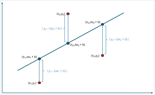
Figure 1 – Graphical representation of the estimated points and fitted curve
The aggregated distance between the actual and estimated values is given by:

that is, by the function:

The minimization of the function S(α, b) can be found by the partial derivatives with respect to α and b:


Dividing the equations by 2 and distributing the sums we will have:


Or even,
 b =
b = 
 b =
b = 
Note that the 1st equation is simply the 2nd equation multiplied by xi. We can also write the system in matrix form:
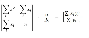
Figure 2 – Matrix representation of the system of equations
To explain the solution, we will call the first matrix X, the second b, and the resultant y, that is, we will represent the system of equations in its matrix form: Xb = y.
Remembering that xi and yi are known points, we can solve the system using Cramer's rule, that is, given Xb = y, we have that the column vector b is solved by:
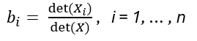
Where Xi is the matrix formed by the substitution
of the i-th column of X by the vector y. In this simple case, we have
a 1st degree linear equation, where we assume that  . But what is the
solution in cases where the analyzed curve takes other forms, such as,
for example, the average production cost curve, similar to a parabola? In these
cases, the equation would take the following form:
. But what is the
solution in cases where the analyzed curve takes other forms, such as,
for example, the average production cost curve, similar to a parabola? In these
cases, the equation would take the following form:  , right?
Well, simple. Just like in the previous example, we would
only need to find the coefficients, since the values of xi and yi
are given. Additionally to the previous example, instead of solving a
system of equations with two terms, where the second equation is multiplied by
x, we will have a system of equations with 3 terms, where the third equation is
simply the first multiplied by  .
.
In summary, instead of solving just:
 b =
b =
b =
We will have to solve the new system:
b + n.c =
 b +
b +  =
=
 b +
b +  =
= 
Notice that the 2nd equation is simply the 1st
equation multiplied by x and that the third equation is the second equation
multiplied by (or the first multiplied by ). And, similarly,
we can find the solution using Cramer's rule.
Let's see some practical examples in Excel
1 – Adjusted 1st degree equations
We will start with the simplest example, where the equation represents only a line. Suppose you access your sales system and capture the historical demand for a product. You need to project the demand for the next 3 months.
Below is the graphical representation of the collected points:
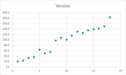
The historical sales refer to the last 18 months and, clearly, there is a growth trend for the upcoming months. We will fit an equation that represents this curve and then estimate the values for the next 3 months. Below is the table of this data in Excel:
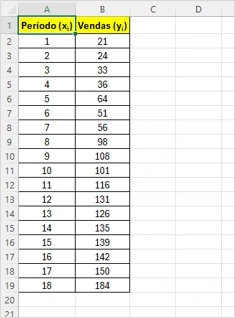
Notice that xi and yi are the
historical data. What we need to do now is find the coefficient that fits
these two variables to the equation yi = αxi + b. What
will we need? According to the matrix resolution shown earlier
(Figure 2), we will need to obtain  , ,
, ,  and from these 18 observations. We will calculate the totals
in row 20 of the spreadsheet.
and from these 18 observations. We will calculate the totals
in row 20 of the spreadsheet.
So we have:
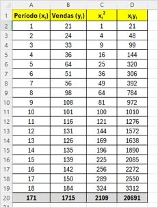
Let's create a small table with the matrix form of the system of equations. This will help us keep the spreadsheet visually aligned with the theory presented earlier.
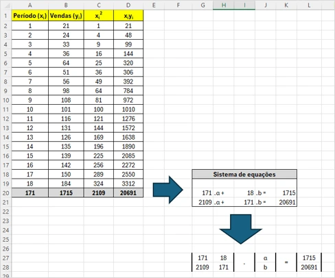
Next, we will use Cramer's rule to calculate the coefficients α and b. We will do this just below the matrices. We will then calculate the coefficients in cells L31 and L35 using the formula =MATRIX.DETERM().
The determinant of matrix X is equal to -8721. We found this result using the formula: =MATRIX.DETERM(G27:H28).
To calculate the coefficients α and b, we should only divide the determinants of the altered matrices by the value -8721.
Below are the formulas and the respective results:
α -> =MATRIX.DETERM(H30:I31) /-8271 = 9.08
b -> =MATRIX.DETERM(H34:I35) / -8271 = 9.03
Finally, we can now calculate the estimated values for periods 19, 20, and 21 (rounded values):
Period 19 -> (9.08*19) + 9.03 = 182
Period 20 -> (9.08*20) + 9.03 = 191
Period 21 -> (9.08*21) + 9.03 = 200
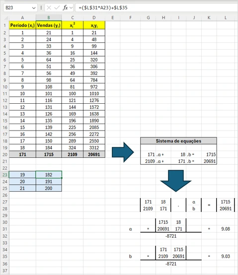
Figure 3 – Spreadsheet for calculating coefficients α and b and estimated values
2 – Adjusted quadratic equations
Let's move on to a slightly more elaborate problem that includes optimization.
This time you capture data on total costs and quantities produced from a work center, as shown in the figure below. You need to find the optimal quantity of production.
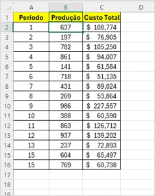
Let’s initially recall the economic theory of diminishing returns. This theory states that after an optimal capacity level is reached, adding a factor of production will result in smaller increases in production. In other words, the marginal cost of production becomes greater than the average cost and the average cost curve becomes increasing.
That said, we will create an additional column with the average production cost. And, for better visualization of the cost behavior, we will sort the table by the column Production.
Below is the table with the processed data and the respective graph of the average cost curve.
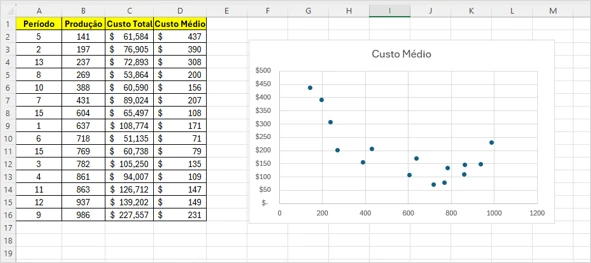
Aligned with the theory of diminishing returns, the average cost curve has a parabolic shape, with an inflection point close to 700 units produced. This behavior may be explained by capacity constraints and, from this point, it may require overtime, subcontracting more expensive producers, etc.
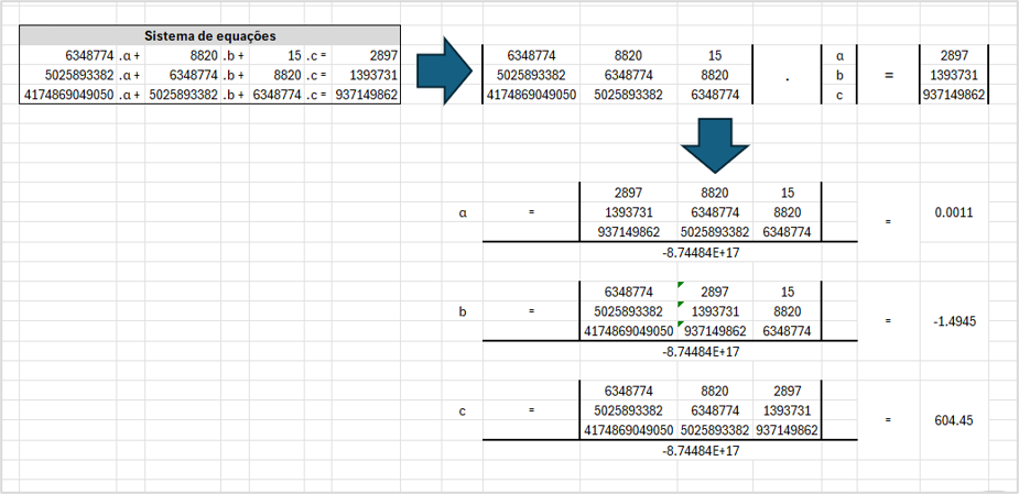
We will use the mentioned system for a 2nd degree polynomial, that is, this time we will need to solve the system of equations:
b +
n.c =
b + =
b + =
Being  the production and
  the
average cost.
the
average cost.
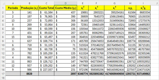
Which leads us to the system of equations and its respective matrix form:
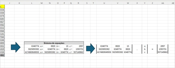
And calculating the coefficients, we will have the following values for α, b and c:
α = 0.0011, b = -1.4945 and c = 604.45
Let's take a look at the graph with the actual values and the regressed values (yi x ӯi):
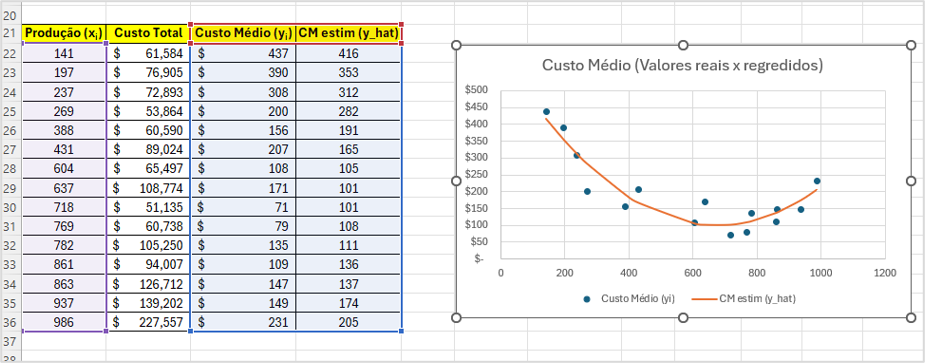
The regression equation indicates that the estimated average cost is given by:

Which has its minimum point given by:

In other words, the minimum point is reached when production is approximately 677 units. At this point, the average production cost is approximately $98.9 / unit.
3 – Adjusted multivariate functions
The solution of the system of equations can be used for functions with multiple
independent variables. Example: the demand for a product that depends not
only on price but also on some attribute of the product and/or market
condition. Assuming that price is xi, durability wi, and the exchange rate
of the dollar zi, the function F(x, w, z) would take the following form:  .
.
And we have to solve:


The 2nd equation is simply the first multiplied by x, the 3rd is the first multiplied by w, and the 4th equation is the first multiplied by z. Similarly, we would need to use Cramer's rule to solve the matrix system:
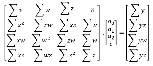
It is common in econometrics to find functions with multiple independent variables. The graphic representation is somewhat compromised, as it is difficult to imagine a graph with more than 3 dimensions. One way to represent them would be to use different characteristics for each point, for example, a bubble chart, where the size of the bubble represents the quantity of a variable. Colors are also useful, as we can associate cooler colors with lower values and warmer colors with higher values.
We will not exemplify cases like this because Excel is, in a way, limited in producing graphs. More sophisticated statistical software, such as R or Python, are more appropriate for this need.
4 – Other curves that can be fitted by regression
We have already seen how versatile this technique is. However, we will not extend the explanations further, we will only exemplify other possibilities of application.
4.1 – Calculation of holding cost based on inventory volume.
Idle stock means a financial cost, right? In many companies, the volume of receipts is high at the beginning of the month, aiming to meet production and is low at the end of the month, aiming for accounting reduction in the stock account.
One way to calculate the financial loss from idle stock during the month would be: to find the function that represents the daily stock levels, calculate the definite integral (0 to 30) of this function and multiply that value by the company's cost of capital. Below is a graphical example of an adjusted equation of a company's stock.
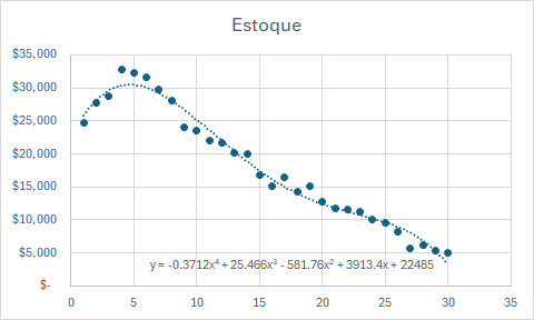
The volume in $ of the stock would be given by:

4.2 – Exponential functions
It is not possible
to use linear regression to fit exponential functions. However, it is possible
to linearize the response variable and, subsequently, find the adjusted model.
A variable with exponential growth, for example  , will have a
linear growth if we use the log of this variable, which will be given by ln() or xln(and).
, will have a
linear growth if we use the log of this variable, which will be given by ln() or xln(and).
5 – Conclusion
Linear regression is an extremely useful technique in predictive data analysis. The use in conjunction with other techniques, such as optimization, makes this technique even more robust, as it extends the use of these models to prescriptive data analysis.
Finally, as already mentioned, if I could give advice to newcomers in the market, I would suggest that they understand well the applicability of this technique, as, in the market, no one finds a problem ready to be solved. You will only find data!