
When flipping a coin once, what is the probability of getting "heads"?
Easy answer! If the coin is fair, the probability is 50%. In other words, if you bet on heads and get heads, you win; otherwise, you lose. Success or failure, occurrence or non- occurence, making a sale or not — all these outcomes can be represented by the values 0 and 1.
Flipping a coin is just an example of an experiment where you cannot control the probabilities of the outcomes. In the real world, however, many events do not occur randomly or without control over the outcomes; it is about correctly identifying the variables that influence these probabilities. For example, sales volume can be increased by adjusting the product price, improving quality, and investing in advertising, among other actions. Similarly, employee turnover can be managed by identifying key retention incentives and mitigating the factors that drive the turnover. And so on.
In this article, I will present a technique used to identify and estimate these probabilities: the logistic model. With this model, it is possible to identify the variables that most impact the outcomes.
But first, we will address some concepts that introduce and deepen the understanding of this technique.
1. Key concepts and fundamentals
To succeed or not to succeed is a binary outcome that follows what is called a Bernoulli distribution, with probability p of occurring and probability 1-p of not occurring, with the sum of p and 1-p being 1 (100%).
|
Event |
Y |
Probability |
|
Occur |
1 |
Pi |
|
Not occur |
0 |
(1 – Pi) |
|
Total |
100% |
The Bernoulli distribution is a special case of the binomial distribution where a single trial is conducted (i.e., n is equal to 1 for a binomial distribution) and is sometimes expressed in the following way:
 , so:
, so:
- If x=0 =>

- If x=1 =>

The response is a binary variable, but many data scientists use linear regression to estimate these probabilities (0 and 1). Is this a good practice? Obviously, no.
Consider the following linear equation:
Ŷi = β1 + β2Xi + ui, considering E(ui) = 0
If Ŷi is a binary response (0 or 1), the adjusted regression should be:
Ŷi = β1 + β2Xi <=> 0 ≤ Ŷi ≤ 1 or;
P̂i = β1 + β2Xi <=> 0 ≤ P̂i ≤ 1
The equation above represents the linear probability model (LPM) and corresponds to a straight line. In this case, it cannot be ensured that the results (P̂i or Ŷi) will respect the limits [0, 1]. Depending on the value of Xi, Ŷi can be negative or greater than 1, unless the following restrictions are applied:
1 – if Ŷi for negative, 0 is considered as the prediction;
2 – if Ŷi is greater than 1, 1 is considered as the prediction.
Below are the figures that illustrate the MPL without restrictions (a) and with restrictions (b):
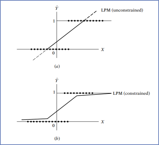
Figure 1: Linear probability models. Source: Basic Econometrics 4th ed. Gujarati
A better way to adequately ensure that the estimated conditional probabilities E(Yi) are between 0 and 1 is to use probit or logit models. Both yield similar results, but, in this article, I will show how to extract useful information from the logit model (or logistic regression model).
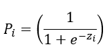
Unlike the linear model, where the probability is a linear transformation of the variable Xi (Pi = β1 + β2Xi), in a logistic regression model, the probabilities of occurrence and non-occurrence are given by:
and
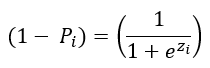
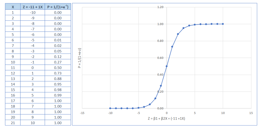
Where the term zi = β1 + β2Xi is called logit.
Note in the figure below that the logit is a linear transformation of X and that the probability function takes the form of a sigmoid curve, varying from -∞ to +∞, with limits in the interval [0, 1].
An interesting metric is called the odds
ratio (odds ratio):  . It represents how much the probability of
occurrence is greater (or lesser) than that of non-occurrence. Thus, for example,
if the probability of occurrence of a sale is 0.8, the probability of non-occurrence will be
0.2. In this case, the odds ratio (odds ratio) is equal to 4, indicating
that the probability of occurrence is four times greater than that of non-
ocurrence. A 50/50 chance (like flipping a coin) results in
an odds ratio of 1. Therefore, if the occurrence is a positive event (like a
sale), the best strategy is to keep this ratio above 1 — that is, with the
probability of sale higher than the probability of no sale.
. It represents how much the probability of
occurrence is greater (or lesser) than that of non-occurrence. Thus, for example,
if the probability of occurrence of a sale is 0.8, the probability of non-occurrence will be
0.2. In this case, the odds ratio (odds ratio) is equal to 4, indicating
that the probability of occurrence is four times greater than that of non-
ocurrence. A 50/50 chance (like flipping a coin) results in
an odds ratio of 1. Therefore, if the occurrence is a positive event (like a
sale), the best strategy is to keep this ratio above 1 — that is, with the
probability of sale higher than the probability of no sale.
Conceptually, the logit is calculated from this metric as the logarithm of the odds ratio (the probability of occurrence divided by the probability of non-occurrence).

Additionally if:

Then:

2. Why is all this important? Interpreting the model
The analysis is quite simple. If the logit represents the logarithm of the odds ratio (odds ratio), we can determine the impact of variable X on the occurrence of an event simply by calculating the exponential of the coefficients (remember: the exponential is also called the antilogarithm).
To facilitate visualization, consider a hypothetical example. Suppose you have a large database with historical customer inquiries, containing records where the customer confirmed the purchase order (1) and others where they did not (0). In this situation, half of the customers purchased their products and the other half did not; therefore, your current odds ratio is 1 (50% / 50%).
You know that you do not operate in a market of homogeneous products (that is, one in which customers do not perceive differences between your products and those of the competition). Thus, in addition to price, it is necessary to identify in the database the relevant variables that lead customers to place orders. Given that your products have a certain degree of differentiation, variables such as durability, warranty, price, capacity, and speed (assuming it is a laptop), as well as other characteristics perceived by customers, should be included in the model. You performed this procedure and, after executing a logistic regression, obtained the following equation:
Sales (yes or no) = -25.93 + 0.3(warranty) + 0.5(durability) - 0.10(price)
To simplify this example, let’s assume that other variables are not statistically significant, only these 3. The warranty is measured in months, durability in years, and price in thousands of dollars.
Question: What do the coefficients indicate about the probability of sales?
Warranty: the coefficient is 0.3, therefore, keeping all
other predictors constant, the probability of a customer confirming the
order increases by 0.3*(0.5*0.5) = 7.5% for each month added to the warranty. The
previous probability will increase from 50% to 57.5%, and the odds ratio
will increase by 35% (0.575/0.425 = 1.35). This increase in the odds ratio is
confirmed by the exponentiation of the coefficient 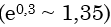 .
.
Durability: the coefficient is 0.5, therefore, keeping all
other predictors constant, the probability of a customer confirming the
order increases by 0.5*(0.5*0.5) = 12.5% for each year added to
durability. The previous probability will increase from 50% to 62.5%, and the odds
ratio will increase by 66% (0.625/0.375 = 1.66). This increase in the odds
ratio is confirmed by the exponentiation of the coefficient 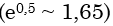 .
.
Price: in this case, the coefficient is negative (-0.10),
therefore, keeping all other predictors constant, the probability of a
customer confirming the order decreases by -0.1*(0.5*0.5) = -2.5% for each thousand
dollars added to the product price. The previous probability will decrease from
50% to 47.5%, and the odds ratio will decrease by 10% (0.475/0.525 = 0.90). This
decrease in the odds ratio is confirmed by the exponentiation of the coefficient
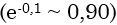 .
.
Note that this is a cold analysis with hypothetical numbers, just to contextualize how powerful logistic regression is. In our example, the improvement in quality may cause a price increase and the results in sales would be a net percentage considering the increases in durability and price. Another point: the improvement in durability may also compromise its own demand (the products last longer), so instead of a good result, you may have the opposite (a decrease in the number of orders made by your customers).
3. Other examples of model application (example included)
There are many other examples of application of this technique; here are a few:
- - Credit risk analysis, based on customer income, past defaults, current debt value, etc.
- - Employee turnover, based on job satisfaction, monthly income, overtime, distance from home, etc.
- - Evaluation of products, such as, for example, the quality of wine based on physical-chemical characteristics (Wine Quality - UCI Machine Learning Repository). In this case, the response variable ranges from 1 to 10, so it is not binomial. If you need to predict the probabilities of different possible outcomes (i.e., more than 2 outcomes) based on independent variables, you should consider a multinomial logistic regression.
Even so, we will use the wine quality database to simulate an example of the impact of characteristics on product sales.
Example with the wine quality dataset from the UCI repository.
The wine quality database will be used as an example. It is publicly available in the UCI ML repository and can be easily accessed using the library ucimlrepo in Python. The database contains 6,497 records (distinct wines) with 11 distinct characteristics (variables): fixed acidity, volatile acidity, citric acid, residual sugar, chlorides, free sulfur dioxide, total sulfur dioxide, density, pH, sulfates, and alcohol content. The target variable is the quality of the wine, assessed by experts on a scale from 0 to 10. An important point about this dataset is that, due to privacy and logistical issues, only physical-chemical (inputs) and sensory (the output) variables are available; that is, there is no data on grape types, wine brand, selling price, etc.
Below, the distribution of each variable (characteristics and target) is presented:
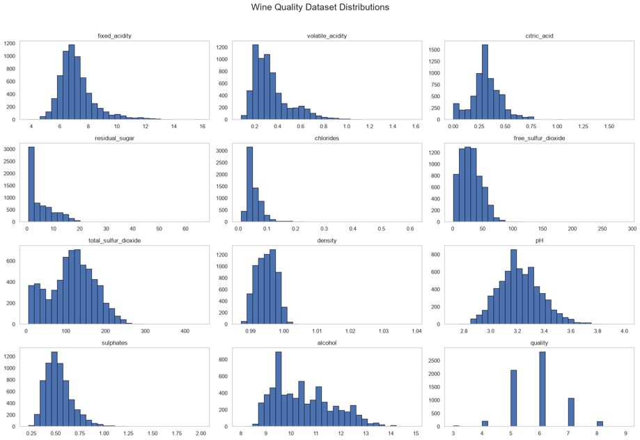
To create our simulation, we will transform the quality into a binary variable. One can imagine that, depending on the score, the wine can be classified as "good or bad taste", "approved or not approved" or "sold or not sold". In our case, we will consider quality results from 0 to 5 as "Do Not Sell" and from 6 to 10 as "Sell".
Results
After the outlier detection and exclusion (used Mahalanobis distance), 6,334 of the 6,497 initial records (wines) were selected – 2,297 classified as "0" and 4,037 classified as "1". This means:
P = 0.637 (63.7%)
(1-P) = 0.363 (36.3%) and,
Odds ratio (odds ratio) = 1.758.
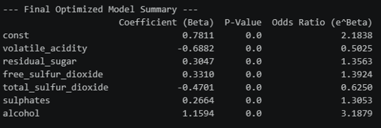
The database was divided into "training" (5,067 records) and "testing" (1,267 records). Both subsets have a similar odds ratio to the original dataset. After running the model on the "training" subset, 5 variables were not statistically significant: chlorides, density, fixed acidity, pH, and citric acid. The results of the remaining variables are presented below:
Model Accuracy
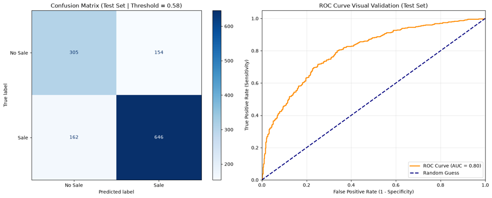
By comparing the actual values of the test dataset with the estimated outputs (y_hat) using a threshold of 0.58, the model achieved 75% accuracy, with 80% True Positives and 34% False Positives. Below, the confusion matrix and the ROC curve are presented.
Analysis
Let's analyze two regression coefficients.
What the new odds ratio (odds ratio) of volatile acidity indicate? It has a negative value of -0.6882, indicating a negative impact on P (Sales). This means that if we add one unit of volatile acidity to the wine, the odds ratio will drop by 50.25%: from the initial value of 1.758 to about 0.883. P will decrease from 63.7% to about 46.9% and, consequently, (1-P) will increase from 36.3% to 53.1%.
On the other hand, alcohol content is the variable that has the most positive impact on quality. The new odds ratio will increase by about 219%: from the initial value of 1.758 to approximately 5.603 (1.758 * 3.1879). Thus, P will increase from 63.7% to about 84.9%, and (1-P) will decrease from 36.3% to 15.1%.
Is notorious that the specialists highly consider alcoholic composition as a very positive characteristic while volatile acidity as a very negative characteristic.
Conclusion
Logistic regression is a powerful and easily interpretable tool that can be applied across various fields, such as finance, HR, or supply chain management. New product launches are often based on simple improvements to existing products (e.g., a new product offering better performance). In such cases, this methodology proves to be a powerful tool for corporate sales strategies.